Parameters vs FLOPs: Scaling Laws for Optimal Sparsity for Mixture-of-Experts Language Models

📝 Paper Summary

Scaling Laws Efficient Deep Learning

For a fixed compute budget, increasing the total parameter count while proportionally increasing sparsity in Mixture-of-Experts models consistently yields better pretraining performance than denser counterparts.

Core Problem

Traditional scaling laws use parameter count as a proxy for compute, but sparse Mixture-of-Experts (MoE) models decouple these factors, making it unclear how to optimally trade off total parameters vs. active parameters (FLOPs per token) under a fixed budget.

Why it matters:

Current laws don't account for 'FLOP-free' parameters in MoEs, leading to suboptimal resource allocation during pretraining.
Understanding this trade-off allows training larger models that are cheaper to infer, maximizing efficiency for both training and deployment.
Designers need a recipe to balance memory (total parameters) and speed (active parameters) to get the best loss for a given compute budget.

Concrete Example: When training a model with a fixed FLOP budget, a standard dense model might be restricted to 7B parameters. An MoE could use 50B parameters with high sparsity (only activating 7B per token). Without updated scaling laws, it's unknown if the 50B sparse model outperforms the 7B dense model or if extreme sparsity degrades learning efficiency.

Key Novelty

IsoFLOP Scaling Laws for MoE Sparsity

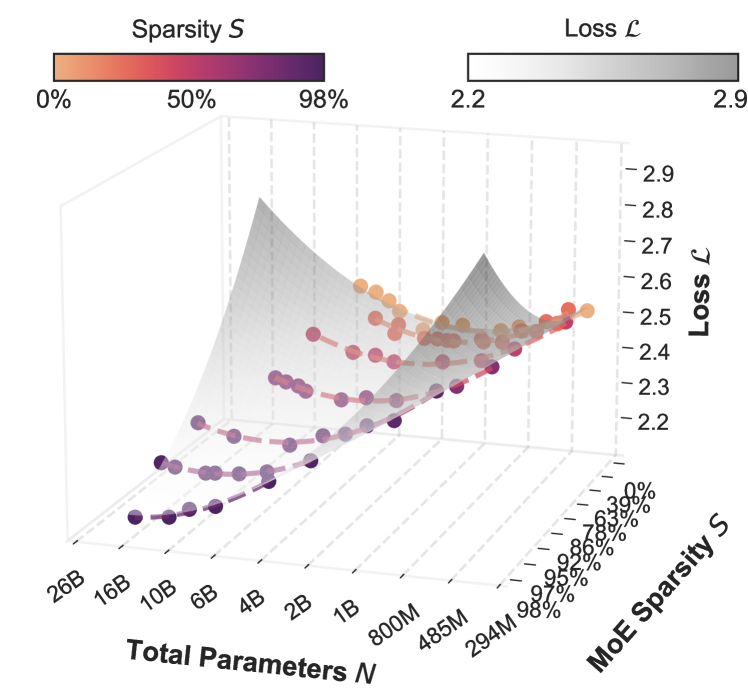
Fits a 3D 'IsoFLOP surface' to model loss as a function of total parameters and sparsity level under a fixed compute budget.
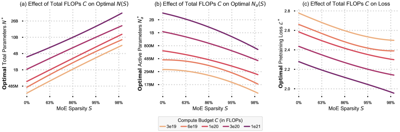
Demonstrates that optimal sparsity approaches 1.0 as model size grows: it is always beneficial to add more experts (increasing total parameters) while keeping active parameters low.
Introduces a modified parametric scaling law equation that explicitly includes a sparsity term to predict loss without needing MoE-specific hyperparameter counts.

Architecture

3D IsoFLOP Surface plotting Loss vs. Model Size (N) vs. Sparsity (S) for a fixed compute budget.

Evaluation Highlights

Optimal sparsity level approaches 1.0 across all compute budgets, meaning larger, sparser models consistently beat denser ones in pretraining perplexity.
For a fixed model size, performance follows a parabolic curve with respect to sparsity, revealing a distinct 'optimal sparsity' point that increases with model size.
On downstream tasks like language understanding, sparse models match dense models with equal pretraining perplexity, though they may lag on reading comprehension due to lower inference-time compute.

Breakthrough Assessment

7/10

Provides crucial empirical scaling laws for MoEs, resolving the ambiguity of parameter vs. compute scaling. The finding that 'sparser is always better' for pretraining is strong, though downstream caveats apply.

⚙️ Technical Details

Problem Definition

Setting: Language Modeling (Next Token Prediction) with Sparse Mixture-of-Experts Transformers

Inputs: Tokenized text sequences

Outputs: Probability distribution over the next token

Pipeline Flow

Input Tokens
MoE Transformer Layers (Router selects Top-K experts)
Output Logits
Loss Calculation

System Modules

MoE Transformer Block

Process tokens using a sparse subset of available parameters

Model or implementation: Sparse Mixture-of-Experts Transformer

Novel Architectural Elements

Analysis focuses on the 'Sparsity' hyperparameter S as a primary scaling dimension alongside N (parameters) and D (data)

Modeling

Base Model: Sparse Mixture-of-Experts Transformer

Training Method: Pretraining (Next Token Prediction)

Objective Functions:

Purpose: Minimize prediction error.

Formally: Cross-Entropy Loss on next token prediction.

Key Hyperparameters:

optimizer: AdamW (implied by standard transformer training, specific values not in text)
loss_delta_huber: 10^-3 (for fitting scaling laws)

Compute: Not explicitly reported in the paper (focus is on theoretical FLOPs/scaling laws rather than wall-clock time)

Comparison to Prior Work

vs. Chinchilla: Extends IsoFLOP analysis to 3D by adding Sparsity as a dimension, finding separate optima for total vs. active parameters
vs. Ludziejewski et al.: Focuses specifically on the trade-off between total parameters and FLOPs per example via sparsity, rather than just expert count/granularity

Limitations

Analysis ignores memory bandwidth and communication overheads, which are significant for MoEs
Downstream evaluation is limited to few-shot settings; full finetuning behavior is unexplored
Specific hardware constraints (e.g., GPU memory limits) are abstracted away by using theoretical FLOPs
Experiments likely at smaller scales compared to production LLMs (exact scales not detailed in snippet)

Reproducibility

The paper provides the parametric scaling law equation and the methodology for fitting it (IsoFLOP surface). Specific code URLs or model weights are not provided in the text.

📊 Experiments & Results

Evaluation Setup

Language Modeling Pretraining and Downstream Few-Shot Evaluation

Benchmarks:

Validation Loss (Language Modeling (Perplexity))
LLM-Foundry Suite (Downstream Tasks (Language Understanding, World Knowledge, Reading Comprehension, Symbolic Reasoning))

Metrics:

Pretraining Loss
Downstream Task Error/Accuracy
Statistical methodology: Fit 3D polynomial surfaces to empirical data; Grid search for optimal scaling coefficients.

Key Results

Benchmark	Metric	Baseline	This Paper	Δ
IsoFLOP analysis reveals the relationship between model size, sparsity, and loss under fixed compute.
IsoFLOP Surface	Cross-Validation Error	Not reported in the paper	Lowest with degree (2,2,2)	Not reported in the paper
Synthetic/Pretraining Data	Optimal Sparsity Level	0.0	Approaches 1.0	+1.0

Experiment Figures

Slices of the IsoFLOP surface. (a) Loss vs Sparsity for fixed N. (b) Loss vs N for fixed S.

Scatter plots of Downstream Performance vs. Upstream Loss for various tasks, colored by sparsity.

Main Takeaways

Pretraining: Increasing model capacity via parameters (N) is more beneficial than increasing FLOPs per example (active parameters), provided sparsity is optimized.
Fixed Compute: For a fixed FLOP budget, the compute-optimal model size grows as sparsity increases, but the active parameter count decreases.
Fixed Model Size: If N is constrained (e.g., memory limits), there exists a distinct optimal sparsity level S* that balances capacity and token throughput.
Downstream Transfer: For most tasks, upstream perplexity predicts downstream performance regardless of sparsity. Exception: Reading comprehension (e.g., SQuAD), where sparser models underperform denser ones at the same perplexity, likely due to insufficient inference-time compute.

📚 Prerequisite Knowledge

Prerequisites

Scaling Laws (Kaplan et al., Hoffmann et al.)
Mixture-of-Experts (MoE) architecture
FLOPs (Floating Point Operations) estimation
Perplexity / Cross-Entropy Loss

Key Terms

MoE: Mixture-of-Experts—a neural network architecture where different subsets of the model (experts) are activated for different inputs

Sparsity (S): The ratio of inactive experts to the total number of experts; higher sparsity means a smaller fraction of the model is used per token

IsoFLOP: A curve or surface representing constant computational cost (FLOPs), used to find optimal hyperparameters for that specific budget

Active Parameters (N_a): The number of parameters actually used to process a single token; determines inference cost and FLOPs per example

Total Parameters (N): The sum of all weights in the model, including those not activated for a given token; determines memory usage

CoT: Chain-of-Thought—a prompting strategy where the model generates intermediate reasoning steps, effectively increasing compute per example during inference

Upstream Performance: Performance on the pretraining objective (usually next-token prediction loss or perplexity)

Downstream Performance: Performance on specific tasks (e.g., QA, reasoning) often measured via few-shot prompting after pretraining